ArviZ migration guide

We have been working on refactoring ArviZ to allow more flexibility and extensibility of its elements while keeping as much as possible a friendly user-interface that gives sensible results with little to no arguments.

One important change is enhanced modularity. Everything will still be available through a common namespace arviz, but ArviZ will now be composed of 3 smaller libraries:

• arviz-base data related functionality, including converters from different PPLs.

• arviz-stats for statistical functions and diagnostics.

• arviz-plots for visual checks built on top of arviz-stats and arviz-base.

Each library depends only on a minimal set of libraries, with a lot of functionality built on top of optional dependencies. This keeps ArviZ smaller and easier to install as you can install only the components you really need. The main examples are:

• arviz-base has no I/O library as a dependency, but you can use netcdf4, h5netcdf or zarr to read and write your data, allowing you to install only the one you need.

• arviz-plots has no plotting library as a dependency, but it can generate plots with matplotlib, bokeh or plotly if they are installed.

At the time of writing, arviz-xyz libraries are independent of the arviz library, but arviz tries to import the arviz-xyz libraries and exposes all their elements through the arviz.preview namespace. In the future, with the ArviZ 1.0 release, the arviz namespace will look like arviz.preview looks like today.

We encourage you to try it out and get a head start on the migration!

import arviz.preview as az
# change to import arviz as az after ArviZ 1.0 release

Check all 3 libraries have been exposed correctly:

print(az.info)

arviz_base available, exposing its functions as part of arviz.preview
arviz_stats available, exposing its functions as part of arviz.preview
arviz_plots available, exposing its functions as part of arviz.preview

arviz-base

DataTree

One of the main differences is the arviz.InferenceData object doesn’t exist any more. arviz-base uses xarray.DataTree instead. This is a new data structure in xarray, so it might still have some rough edges, but it is much more flexible and powerful. To give some examples, I/O will now be more flexible, and any format supported by xarray is automatically available to you, no need to add wrappers on top of them within ArviZ. It is also possible to have arbitrary nesting of variables within groups and subgroups.

Important

Not all the functionality on xarray.DataTree will be compatible with ArviZ as it would be too much work for us to cover and maintain. If there are things you have always wanted to do but were not possible with InferenceData and are now possible with DataTree please try them out, give feedback on them and on desired behaviour for things that still don’t work. After a couple releases the “ArviZverse” will stabilize much more and it might not be possible to add support for that anymore.

I already have InferenceData object from an external library

InferenceData already has a method to convert it to DataTree.

import arviz as arviz_legacy

idata = arviz_legacy.load_arviz_data("centered_eight")

idata.to_datatree()

<xarray.DatasetView> Size: 0B
Dimensions:  ()
Data variables:
    *empty*

xarray.DataTree

• Groups: (8)
  (6/8)
  <xarray.DatasetView> Size: 165kB
  Dimensions:  (chain: 4, draw: 500, school: 8)
  Coordinates:
    * chain    (chain) int64 32B 0 1 2 3
    * draw     (draw) int64 4kB 0 1 2 3 4 5 6 7 ... 493 494 495 496 497 498 499
    * school   (school) <U16 512B 'Choate' 'Deerfield' ... 'Mt. Hermon'
  Data variables:
      mu       (chain, draw) float64 16kB ...
      theta    (chain, draw, school) float64 128kB ...
      tau      (chain, draw) float64 16kB ...
  Attributes:
      created_at:                 2022-10-13T14:37:37.315398
      arviz_version:              0.13.0.dev0
      inference_library:          pymc
      inference_library_version:  4.2.2
      sampling_time:              7.480114936828613
      tuning_steps:               1000

  posterior

  • Groups: (0)
  • Dimensions:
    • chain: 4
    • draw: 500
    • school: 8
  • Coordinates: (3)
    • chain
      (chain)
      int64
      0 1 2 3

      array([0, 1, 2, 3])

    • draw
      (draw)
      int64
      0 1 2 3 4 5 ... 495 496 497 498 499

      array([  0,   1,   2, ..., 497, 498, 499], shape=(500,))

    • school
      (school)
      <U16
      'Choate' ... 'Mt. Hermon'

      array(['Choate', 'Deerfield', 'Phillips Andover', 'Phillips Exeter',
             'Hotchkiss', 'Lawrenceville', "St. Paul's", 'Mt. Hermon'], dtype='<U16')

  • Data variables: (3)
    • mu
      (chain, draw)
      float64
      ...

      [2000 values with dtype=float64]

    • theta
      (chain, draw, school)
      float64
      ...

      [16000 values with dtype=float64]

    • tau
      (chain, draw)
      float64
      ...

      [2000 values with dtype=float64]

  • Attributes: (6)

    created_at :

    2022-10-13T14:37:37.315398

    arviz_version :

    0.13.0.dev0

    inference_library :

    pymc

    inference_library_version :

    4.2.2

    sampling_time :

    7.480114936828613

    tuning_steps :

    1000

  <xarray.DatasetView> Size: 133kB
  Dimensions:  (chain: 4, draw: 500, school: 8)
  Coordinates:
    * chain    (chain) int64 32B 0 1 2 3
    * draw     (draw) int64 4kB 0 1 2 3 4 5 6 7 ... 493 494 495 496 497 498 499
    * school   (school) <U16 512B 'Choate' 'Deerfield' ... 'Mt. Hermon'
  Data variables:
      obs      (chain, draw, school) float64 128kB ...
  Attributes:
      arviz_version:              0.13.0.dev0
      created_at:                 2022-10-13T14:37:41.460544
      inference_library:          pymc
      inference_library_version:  4.2.2

  posterior_predictive

  • Groups: (0)
  • Dimensions:
    • chain: 4
    • draw: 500
    • school: 8
  • Coordinates: (3)
    • chain
      (chain)
      int64
      0 1 2 3

      array([0, 1, 2, 3])

    • draw
      (draw)
      int64
      0 1 2 3 4 5 ... 495 496 497 498 499

      array([  0,   1,   2, ..., 497, 498, 499], shape=(500,))

    • school
      (school)
      <U16
      'Choate' ... 'Mt. Hermon'

      array(['Choate', 'Deerfield', 'Phillips Andover', 'Phillips Exeter',
             'Hotchkiss', 'Lawrenceville', "St. Paul's", 'Mt. Hermon'], dtype='<U16')

  • Data variables: (1)
    • obs
      (chain, draw, school)
      float64
      ...

      [16000 values with dtype=float64]

  • Attributes: (4)

    arviz_version :

    0.13.0.dev0

    created_at :

    2022-10-13T14:37:41.460544

    inference_library :

    pymc

    inference_library_version :

    4.2.2

  <xarray.DatasetView> Size: 133kB
  Dimensions:  (chain: 4, draw: 500, school: 8)
  Coordinates:
    * chain    (chain) int64 32B 0 1 2 3
    * draw     (draw) int64 4kB 0 1 2 3 4 5 6 7 ... 493 494 495 496 497 498 499
    * school   (school) <U16 512B 'Choate' 'Deerfield' ... 'Mt. Hermon'
  Data variables:
      obs      (chain, draw, school) float64 128kB ...
  Attributes:
      arviz_version:              0.13.0.dev0
      created_at:                 2022-10-13T14:37:37.487399
      inference_library:          pymc
      inference_library_version:  4.2.2

  log_likelihood

  • Groups: (0)
  • Dimensions:
    • chain: 4
    • draw: 500
    • school: 8
  • Coordinates: (3)
    • chain
      (chain)
      int64
      0 1 2 3

      array([0, 1, 2, 3])

    • draw
      (draw)
      int64
      0 1 2 3 4 5 ... 495 496 497 498 499

      array([  0,   1,   2, ..., 497, 498, 499], shape=(500,))

    • school
      (school)
      <U16
      'Choate' ... 'Mt. Hermon'

      array(['Choate', 'Deerfield', 'Phillips Andover', 'Phillips Exeter',
             'Hotchkiss', 'Lawrenceville', "St. Paul's", 'Mt. Hermon'], dtype='<U16')

  • Data variables: (1)
    • obs
      (chain, draw, school)
      float64
      ...

      [16000 values with dtype=float64]

  • Attributes: (4)

    arviz_version :

    0.13.0.dev0

    created_at :

    2022-10-13T14:37:37.487399

    inference_library :

    pymc

    inference_library_version :

    4.2.2

  ...

  <xarray.DatasetView> Size: 37kB
  Dimensions:  (chain: 1, draw: 500, school: 8)
  Coordinates:
    * chain    (chain) int64 8B 0
    * draw     (draw) int64 4kB 0 1 2 3 4 5 6 7 ... 493 494 495 496 497 498 499
    * school   (school) <U16 512B 'Choate' 'Deerfield' ... 'Mt. Hermon'
  Data variables:
      obs      (chain, draw, school) float64 32kB ...
  Attributes:
      arviz_version:              0.13.0.dev0
      created_at:                 2022-10-13T14:37:26.604969
      inference_library:          pymc
      inference_library_version:  4.2.2

  prior_predictive

  • Groups: (0)
  • Dimensions:
    • chain: 1
    • draw: 500
    • school: 8
  • Coordinates: (3)
    • chain
      (chain)
      int64
      0

      array([0])

    • draw
      (draw)
      int64
      0 1 2 3 4 5 ... 495 496 497 498 499

      array([  0,   1,   2, ..., 497, 498, 499], shape=(500,))

    • school
      (school)
      <U16
      'Choate' ... 'Mt. Hermon'

      array(['Choate', 'Deerfield', 'Phillips Andover', 'Phillips Exeter',
             'Hotchkiss', 'Lawrenceville', "St. Paul's", 'Mt. Hermon'], dtype='<U16')

  • Data variables: (1)
    • obs
      (chain, draw, school)
      float64
      ...

      [4000 values with dtype=float64]

  • Attributes: (4)

    arviz_version :

    0.13.0.dev0

    created_at :

    2022-10-13T14:37:26.604969

    inference_library :

    pymc

    inference_library_version :

    4.2.2

  <xarray.DatasetView> Size: 576B
  Dimensions:  (school: 8)
  Coordinates:
    * school   (school) <U16 512B 'Choate' 'Deerfield' ... 'Mt. Hermon'
  Data variables:
      obs      (school) float64 64B ...
  Attributes:
      arviz_version:              0.13.0.dev0
      created_at:                 2022-10-13T14:37:26.606375
      inference_library:          pymc
      inference_library_version:  4.2.2

  observed_data

  • Groups: (0)
  • Dimensions:
    • school: 8
  • Coordinates: (1)
    • school
      (school)
      <U16
      'Choate' ... 'Mt. Hermon'

      array(['Choate', 'Deerfield', 'Phillips Andover', 'Phillips Exeter',
             'Hotchkiss', 'Lawrenceville', "St. Paul's", 'Mt. Hermon'], dtype='<U16')

  • Data variables: (1)
    • obs
      (school)
      float64
      ...

      [8 values with dtype=float64]

  • Attributes: (4)

    arviz_version :

    0.13.0.dev0

    created_at :

    2022-10-13T14:37:26.606375

    inference_library :

    pymc

    inference_library_version :

    4.2.2

  <xarray.DatasetView> Size: 576B
  Dimensions:  (school: 8)
  Coordinates:
    * school   (school) <U16 512B 'Choate' 'Deerfield' ... 'Mt. Hermon'
  Data variables:
      scores   (school) float64 64B ...
  Attributes:
      arviz_version:              0.13.0.dev0
      created_at:                 2022-10-13T14:37:26.607471
      inference_library:          pymc
      inference_library_version:  4.2.2

  constant_data

  • Groups: (0)
  • Dimensions:
    • school: 8
  • Coordinates: (1)
    • school
      (school)
      <U16
      'Choate' ... 'Mt. Hermon'

      array(['Choate', 'Deerfield', 'Phillips Andover', 'Phillips Exeter',
             'Hotchkiss', 'Lawrenceville', "St. Paul's", 'Mt. Hermon'], dtype='<U16')

  • Data variables: (1)
    • scores
      (school)
      float64
      ...

      [8 values with dtype=float64]

  • Attributes: (4)

    arviz_version :

    0.13.0.dev0

    created_at :

    2022-10-13T14:37:26.607471

    inference_library :

    pymc

    inference_library_version :

    4.2.2

• Dimensions:
• Coordinates: (0)
• Inherited coordinates: (0)
• Data variables: (0)
• Attributes: (0)

What about my existing netcdf/zarr files?

They are still valid. There have been no changes on this end and don’t plan to make any. The only difference is which function handles I/O. There used to be functions in the main arviz namespace like arviz.from_zarr and methods to InferenceData such as .to_netcdf. These are now part of xarray itself:

Function in legacy ArviZ	New equivalent in xarray
arviz.from_netcdf	xarray.open_datatree()[1]
arviz.from_zarr	xarray.open_datatree()[1]
arviz.to_netcdf	-
arviz.to_zarr	-
arviz.InferenceData.from_netcdf	-
arviz.InferenceData.from_zarr	-
arviz.InferenceData.to_netcdf	xarray.DataTree.to_netcdf()
arviz.InferenceData.to_zarr	xarray.DataTree.to_zarr()

Here is an example where we store an InferenceData as a netcdf then read the generated file as is through xarray.open_datatree()

idata.to_netcdf("example.nc")

'example.nc'

from xarray import open_datatree
dt = open_datatree("example.nc")
dt

<xarray.DatasetView> Size: 0B
Dimensions:  ()
Data variables:
    *empty*

xarray.DataTree

• Groups: (8)
  (6/8)
  <xarray.DatasetView> Size: 165kB
  Dimensions:  (chain: 4, draw: 500, school: 8)
  Coordinates:
    * chain    (chain) int64 32B 0 1 2 3
    * draw     (draw) int64 4kB 0 1 2 3 4 5 6 7 ... 493 494 495 496 497 498 499
    * school   (school) <U16 512B 'Choate' 'Deerfield' ... 'Mt. Hermon'
  Data variables:
      mu       (chain, draw) float64 16kB ...
      theta    (chain, draw, school) float64 128kB ...
      tau      (chain, draw) float64 16kB ...
  Attributes:
      created_at:                 2022-10-13T14:37:37.315398
      arviz_version:              0.13.0.dev0
      inference_library:          pymc
      inference_library_version:  4.2.2
      sampling_time:              7.480114936828613
      tuning_steps:               1000

  posterior

  • Groups: (0)
  • Dimensions:
    • chain: 4
    • draw: 500
    • school: 8
  • Coordinates: (3)
    • chain
      (chain)
      int64
      0 1 2 3

      array([0, 1, 2, 3])

    • draw
      (draw)
      int64
      0 1 2 3 4 5 ... 495 496 497 498 499

      array([  0,   1,   2, ..., 497, 498, 499], shape=(500,))

    • school
      (school)
      <U16
      'Choate' ... 'Mt. Hermon'

      array(['Choate', 'Deerfield', 'Phillips Andover', 'Phillips Exeter',
             'Hotchkiss', 'Lawrenceville', "St. Paul's", 'Mt. Hermon'], dtype='<U16')

  • Data variables: (3)
    • mu
      (chain, draw)
      float64
      ...

      [2000 values with dtype=float64]

    • theta
      (chain, draw, school)
      float64
      ...

      [16000 values with dtype=float64]

    • tau
      (chain, draw)
      float64
      ...

      [2000 values with dtype=float64]

  • Attributes: (6)

    created_at :

    2022-10-13T14:37:37.315398

    arviz_version :

    0.13.0.dev0

    inference_library :

    pymc

    inference_library_version :

    4.2.2

    sampling_time :

    7.480114936828613

    tuning_steps :

    1000

  <xarray.DatasetView> Size: 133kB
  Dimensions:  (chain: 4, draw: 500, school: 8)
  Coordinates:
    * chain    (chain) int64 32B 0 1 2 3
    * draw     (draw) int64 4kB 0 1 2 3 4 5 6 7 ... 493 494 495 496 497 498 499
    * school   (school) <U16 512B 'Choate' 'Deerfield' ... 'Mt. Hermon'
  Data variables:
      obs      (chain, draw, school) float64 128kB ...
  Attributes:
      arviz_version:              0.13.0.dev0
      created_at:                 2022-10-13T14:37:41.460544
      inference_library:          pymc
      inference_library_version:  4.2.2

  posterior_predictive

  • Groups: (0)
  • Dimensions:
    • chain: 4
    • draw: 500
    • school: 8
  • Coordinates: (3)
    • chain
      (chain)
      int64
      0 1 2 3

      array([0, 1, 2, 3])

    • draw
      (draw)
      int64
      0 1 2 3 4 5 ... 495 496 497 498 499

      array([  0,   1,   2, ..., 497, 498, 499], shape=(500,))

    • school
      (school)
      <U16
      'Choate' ... 'Mt. Hermon'

      array(['Choate', 'Deerfield', 'Phillips Andover', 'Phillips Exeter',
             'Hotchkiss', 'Lawrenceville', "St. Paul's", 'Mt. Hermon'], dtype='<U16')

  • Data variables: (1)
    • obs
      (chain, draw, school)
      float64
      ...

      [16000 values with dtype=float64]

  • Attributes: (4)

    arviz_version :

    0.13.0.dev0

    created_at :

    2022-10-13T14:37:41.460544

    inference_library :

    pymc

    inference_library_version :

    4.2.2

  <xarray.DatasetView> Size: 133kB
  Dimensions:  (chain: 4, draw: 500, school: 8)
  Coordinates:
    * chain    (chain) int64 32B 0 1 2 3
    * draw     (draw) int64 4kB 0 1 2 3 4 5 6 7 ... 493 494 495 496 497 498 499
    * school   (school) <U16 512B 'Choate' 'Deerfield' ... 'Mt. Hermon'
  Data variables:
      obs      (chain, draw, school) float64 128kB ...
  Attributes:
      arviz_version:              0.13.0.dev0
      created_at:                 2022-10-13T14:37:37.487399
      inference_library:          pymc
      inference_library_version:  4.2.2

  log_likelihood

  • Groups: (0)
  • Dimensions:
    • chain: 4
    • draw: 500
    • school: 8
  • Coordinates: (3)
    • chain
      (chain)
      int64
      0 1 2 3

      array([0, 1, 2, 3])

    • draw
      (draw)
      int64
      0 1 2 3 4 5 ... 495 496 497 498 499

      array([  0,   1,   2, ..., 497, 498, 499], shape=(500,))

    • school
      (school)
      <U16
      'Choate' ... 'Mt. Hermon'

      array(['Choate', 'Deerfield', 'Phillips Andover', 'Phillips Exeter',
             'Hotchkiss', 'Lawrenceville', "St. Paul's", 'Mt. Hermon'], dtype='<U16')

  • Data variables: (1)
    • obs
      (chain, draw, school)
      float64
      ...

      [16000 values with dtype=float64]

  • Attributes: (4)

    arviz_version :

    0.13.0.dev0

    created_at :

    2022-10-13T14:37:37.487399

    inference_library :

    pymc

    inference_library_version :

    4.2.2

  ...

  <xarray.DatasetView> Size: 37kB
  Dimensions:  (chain: 1, draw: 500, school: 8)
  Coordinates:
    * chain    (chain) int64 8B 0
    * draw     (draw) int64 4kB 0 1 2 3 4 5 6 7 ... 493 494 495 496 497 498 499
    * school   (school) <U16 512B 'Choate' 'Deerfield' ... 'Mt. Hermon'
  Data variables:
      obs      (chain, draw, school) float64 32kB ...
  Attributes:
      arviz_version:              0.13.0.dev0
      created_at:                 2022-10-13T14:37:26.604969
      inference_library:          pymc
      inference_library_version:  4.2.2

  prior_predictive

  • Groups: (0)
  • Dimensions:
    • chain: 1
    • draw: 500
    • school: 8
  • Coordinates: (3)
    • chain
      (chain)
      int64
      0

      array([0])

    • draw
      (draw)
      int64
      0 1 2 3 4 5 ... 495 496 497 498 499

      array([  0,   1,   2, ..., 497, 498, 499], shape=(500,))

    • school
      (school)
      <U16
      'Choate' ... 'Mt. Hermon'

      array(['Choate', 'Deerfield', 'Phillips Andover', 'Phillips Exeter',
             'Hotchkiss', 'Lawrenceville', "St. Paul's", 'Mt. Hermon'], dtype='<U16')

  • Data variables: (1)
    • obs
      (chain, draw, school)
      float64
      ...

      [4000 values with dtype=float64]

  • Attributes: (4)

    arviz_version :

    0.13.0.dev0

    created_at :

    2022-10-13T14:37:26.604969

    inference_library :

    pymc

    inference_library_version :

    4.2.2

  <xarray.DatasetView> Size: 576B
  Dimensions:  (school: 8)
  Coordinates:
    * school   (school) <U16 512B 'Choate' 'Deerfield' ... 'Mt. Hermon'
  Data variables:
      obs      (school) float64 64B ...
  Attributes:
      arviz_version:              0.13.0.dev0
      created_at:                 2022-10-13T14:37:26.606375
      inference_library:          pymc
      inference_library_version:  4.2.2

  observed_data

  • Groups: (0)
  • Dimensions:
    • school: 8
  • Coordinates: (1)
    • school
      (school)
      <U16
      'Choate' ... 'Mt. Hermon'

      array(['Choate', 'Deerfield', 'Phillips Andover', 'Phillips Exeter',
             'Hotchkiss', 'Lawrenceville', "St. Paul's", 'Mt. Hermon'], dtype='<U16')

  • Data variables: (1)
    • obs
      (school)
      float64
      ...

      [8 values with dtype=float64]

  • Attributes: (4)

    arviz_version :

    0.13.0.dev0

    created_at :

    2022-10-13T14:37:26.606375

    inference_library :

    pymc

    inference_library_version :

    4.2.2

  <xarray.DatasetView> Size: 576B
  Dimensions:  (school: 8)
  Coordinates:
    * school   (school) <U16 512B 'Choate' 'Deerfield' ... 'Mt. Hermon'
  Data variables:
      scores   (school) float64 64B ...
  Attributes:
      arviz_version:              0.13.0.dev0
      created_at:                 2022-10-13T14:37:26.607471
      inference_library:          pymc
      inference_library_version:  4.2.2

  constant_data

  • Groups: (0)
  • Dimensions:
    • school: 8
  • Coordinates: (1)
    • school
      (school)
      <U16
      'Choate' ... 'Mt. Hermon'

      array(['Choate', 'Deerfield', 'Phillips Andover', 'Phillips Exeter',
             'Hotchkiss', 'Lawrenceville', "St. Paul's", 'Mt. Hermon'], dtype='<U16')

  • Data variables: (1)
    • scores
      (school)
      float64
      ...

      [8 values with dtype=float64]

  • Attributes: (4)

    arviz_version :

    0.13.0.dev0

    created_at :

    2022-10-13T14:37:26.607471

    inference_library :

    pymc

    inference_library_version :

    4.2.2

• Dimensions:
• Coordinates: (0)
• Inherited coordinates: (0)
• Data variables: (0)
• Attributes: (0)

Other key differences

DataTree supports an arbitrary level of nesting (as opposed to the exactly 1 level of nesting in InferenceData). Thus, to keep things consistent accessing its groups returns a DataTree, even if it is a leaf group. This means that dt["posterior"] will now return a DataTree. In many cases this is irrelevant, but there will be some cases where you’ll want the group as a Dataset instead. You can achieve this with dt["posterior"].dataset.

There are no changes at the variable/DataArray level. Thus, dt["posterior"]["theta"] is still a DataArray, accessing its variables is one of the cases where having either DataTree or Dataset is irrelevant.

Enhanced converter flexibility

Were you constantly needing to add an extra axis to your data because it didn’t have any chain dimension? No more!

import numpy as np
rng = np.random.default_rng()
data = rng.normal(size=1000)

# arviz_legacy.from_dict({"posterior": {"mu": data}}) would fail
# unless you did data[None, :] to add the chain dimension
az.rcParams["data.sample_dims"] = "sample"

dt = az.from_dict({"posterior": {"mu": data}})
dt

<xarray.DatasetView> Size: 0B
Dimensions:  ()
Data variables:
    *empty*

xarray.DataTree

• Groups: (1)
  <xarray.DatasetView> Size: 16kB
  Dimensions:  (sample: 1000)
  Coordinates:
    * sample   (sample) int64 8kB 0 1 2 3 4 5 6 7 ... 993 994 995 996 997 998 999
  Data variables:
      mu       (sample) float64 8kB 1.327 -0.6268 -0.4653 ... 0.196 1.796 2.337
  Attributes:
      created_at:                 2025-07-08T23:17:47.604349+00:00
      creation_library:           ArviZ
      creation_library_version:   0.7.0.dev0
      creation_library_language:  Python

  posterior

  • Groups: (0)
  • Dimensions:
    • sample: 1000
  • Coordinates: (1)
    • sample
      (sample)
      int64
      0 1 2 3 4 5 ... 995 996 997 998 999

      array([  0,   1,   2, ..., 997, 998, 999], shape=(1000,))

  • Data variables: (1)
    • mu
      (sample)
      float64
      1.327 -0.6268 ... 1.796 2.337

      array([ 1.32701217e+00, -6.26808828e-01, -4.65295124e-01,  1.72899928e+00,
             -1.25463305e+00,  1.66718092e+00, -3.95729766e-01,  1.40926162e+00,
             -1.16949842e+00,  4.40194817e-01, -2.83847080e-01, -5.31848299e-02,
              3.61772988e-01, -3.38027748e-01, -9.65615209e-01, -1.24718140e+00,
              2.41471216e+00, -4.09722304e-01, -5.72541182e-01,  1.44779327e+00,
             -2.59635529e-01, -5.58619005e-01, -9.88277191e-01,  8.25209416e-01,
             -1.19836889e+00, -2.95220125e-01, -5.49282635e-01,  3.40885877e-01,
             -1.72215172e+00, -1.28681605e+00, -5.08225115e-02,  1.16958849e+00,
             -8.65911532e-01, -1.43337931e-01, -8.02421853e-01,  3.57981015e-01,
             -4.54234662e-01, -7.11577912e-02, -4.39070726e-01, -8.55643964e-01,
              3.98685254e-01,  1.10405309e+00,  3.16063649e-01, -2.24590963e-01,
             -2.28820957e-01,  4.24807836e-01,  1.13718323e+00,  2.13237469e+00,
             -1.66619571e+00, -1.54618345e-01,  1.36557594e+00, -9.27380401e-01,
             -3.35067933e-01, -2.35650889e+00,  2.35075214e-01,  9.40016845e-01,
              2.17279904e+00, -1.06845664e+00,  9.71592271e-02, -7.79933735e-01,
              9.23968661e-01, -1.12258165e-01, -1.65529308e+00, -1.71104005e+00,
             -5.11804120e-01,  2.21801140e-01, -2.26674291e-01, -1.89270921e-01,
              1.22320989e+00, -7.53463943e-01, -9.26455067e-02, -2.46702045e-02,
              8.74207152e-01, -1.28424540e-01,  9.26657840e-01, -9.46230489e-01,
              1.11613897e+00,  3.53352915e-01,  7.58230281e-01,  1.10474050e+00,
      ...
              2.76782681e-02, -1.20295959e+00,  1.83572061e+00, -1.60290958e+00,
              9.63122978e-01,  1.90521883e+00, -1.34872708e-01, -6.22455967e-01,
             -4.23459058e-01, -1.77620961e+00,  1.48957635e-03,  1.56276200e+00,
             -5.11144410e-01,  9.10121629e-02, -3.89529859e-01, -1.47955241e+00,
              4.92205120e-01,  1.14031830e+00,  5.31882112e-01,  9.08165782e-02,
              2.25768449e-01,  1.93452679e-01,  3.81921881e-01,  1.43873830e-01,
             -5.51679363e-01,  4.07718516e-01,  6.20056042e-01, -9.49259011e-02,
              2.52313439e+00, -1.25986577e+00, -5.01205602e-01, -1.78539730e+00,
              1.04455434e+00, -2.76360169e-01,  6.47418284e-01,  3.39442022e-02,
              7.56245494e-01,  4.33675556e-01,  3.89077697e-01, -6.71387156e-02,
              3.02884663e-01,  3.69225390e-01,  2.29406419e-01,  1.12177503e+00,
             -6.47584339e-01,  1.16067162e-01,  7.18919916e-01, -1.61130889e-01,
             -8.16708890e-01, -1.17776336e+00, -4.18416196e-01,  1.53781926e+00,
             -9.16175139e-01, -5.44848166e-01,  1.43733568e-01,  1.36228652e+00,
              9.35446546e-01, -1.49280423e+00, -1.13110892e+00, -1.39699225e+00,
              1.60333160e-02, -1.01189641e+00,  3.47705458e-01, -5.52558490e-01,
             -2.21152820e-01,  4.27315341e-02, -4.96151660e-01, -1.70499781e+00,
              2.20550650e-01, -6.98394816e-01, -4.21112835e-01,  1.18538776e+00,
              1.20698713e+00, -8.00455387e-01,  1.22231247e+00, -9.07523246e-01,
             -1.66611472e+00,  1.95973309e-01,  1.79626104e+00,  2.33735049e+00])

  • Attributes: (4)

    created_at :

    2025-07-08T23:17:47.604349+00:00

    creation_library :

    ArviZ

    creation_library_version :

    0.7.0.dev0

    creation_library_language :

    Python

• Dimensions:
• Coordinates: (0)
• Inherited coordinates: (0)
• Data variables: (0)
• Attributes: (0)

# arviz-stats and arviz-plots also take it into account
az.plot_dist(dt);

Note

It is also possible to modify sample_dims through arguments to the different functions.

New data wrangling features

We have also added multiple functions to help with common data wrangling tasks, mostly from and to xarray.Dataset. For example, you can convert a dataset to a wide format dataframe with unique combinations of sample_dims as its rows, with dataset_to_dataframe():

# back to default behaviour
az.rcParams["data.sample_dims"] = ["chain", "draw"]
dt = az.load_arviz_data("centered_eight")
az.dataset_to_dataframe(dt.posterior.dataset)

	mu	theta[Choate]	theta[Deerfield]	theta[Phillips Andover]	theta[Phillips Exeter]	theta[Hotchkiss]	theta[Lawrenceville]	theta[St. Paul's]	theta[Mt. Hermon]	tau
(0, 0)	7.871796	12.320686	9.905367	14.951615	11.011485	5.579602	16.901795	13.198059	15.061366	4.725740
(0, 1)	3.384554	11.285623	9.129324	3.139263	9.433211	7.811516	2.393088	10.055223	6.176724	3.908994
(0, 2)	9.100476	5.708506	5.757932	10.944585	5.895436	9.992984	8.143327	7.604753	8.767647	4.844025
(0, 3)	7.304293	10.037275	8.809068	9.900924	5.768832	9.062876	6.958424	10.298256	3.155304	1.856703
(0, 4)	9.879675	9.149146	5.764986	7.015397	15.688710	3.097395	12.025763	11.316745	17.046142	4.748409
...	...	...	...	...	...	...	...	...	...	...
(3, 495)	1.542688	3.737751	5.393632	0.487845	4.015486	0.717057	-2.675760	0.415968	-4.991247	2.786072
(3, 496)	1.858580	-0.291737	0.110315	1.468877	-3.653346	1.844292	6.055714	4.986218	9.290380	4.281961
(3, 497)	1.766733	3.532515	2.008901	0.510806	0.832185	2.647687	4.707249	3.073314	-2.623069	2.740607
(3, 498)	3.486112	4.182751	7.554251	4.456034	3.300833	1.563307	1.528958	1.096098	8.452282	2.932379
(3, 499)	3.404464	0.192956	6.498428	-0.894424	6.849020	1.859747	7.936460	6.762455	1.295051	4.461246

2000 rows × 10 columns

Note it is also aware of ArviZ naming conventions in addition to using the sample_dims rcParam. It can be further customized through a labeller argument.

Tip

If you want to convert to a long format dataframe, you should use xarray.Dataset.to_dataframe() instead.

arviz-stats

Stats and diagnostics related functionality have also had some changes, and it should also be noted that out of the 3 new modular libraries it is currently the one lagging behind a bit more. At the same time, it does already have several new features that won’t be added to legacy ArviZ at any point, check out its API reference page for the complete and up to date list of available functions.

dim and sample_dims

Similarly to the rest of the libraries, most functions take an argument to indicate which dimensions should be reduced (or considered core dims) in the different computations. Given arviz-stats is the one with behaviour and API closest to xarray itself, this argument can either be dim or sample_dims as a way to keep the APIs of ArviZ and xarray similar.

Let’s see the differences in action. ess uses sample_dims. This means we can do:

dt = az.load_arviz_data("non_centered_eight")
az.ess(dt, sample_dims=["chain", "draw"])

<xarray.DatasetView> Size: 656B
Dimensions:  (school: 8)
Coordinates:
  * school   (school) <U16 512B 'Choate' 'Deerfield' ... 'Mt. Hermon'
Data variables:
    mu       float64 8B 1.65e+03
    theta_t  (school) float64 64B 2.058e+03 2.51e+03 ... 2.455e+03 2.757e+03
    tau      float64 8B 1.115e+03
    theta    (school) float64 64B 1.942e+03 2.199e+03 ... 2.079e+03 2.106e+03

xarray.DataTree

• Groups: (0)
• Dimensions:
  • school: 8
• Coordinates: (1)
  • school
    (school)
    <U16
    'Choate' ... 'Mt. Hermon'

    array(['Choate', 'Deerfield', 'Phillips Andover', 'Phillips Exeter',
           'Hotchkiss', 'Lawrenceville', "St. Paul's", 'Mt. Hermon'], dtype='<U16')

• Inherited coordinates: (0)
• Data variables: (4)
  • mu
    ()
    float64
    1.65e+03

    array(1650.38780995)

  • theta_t
    (school)
    float64
    2.058e+03 2.51e+03 ... 2.757e+03

    array([2058.46200651, 2509.99931608, 2279.05011766, 2211.41168547,
           1907.05837537, 2395.29357483, 2455.48721995, 2756.90062971])

  • tau
    ()
    float64
    1.115e+03

    array(1115.42920146)

  • theta
    (school)
    float64
    1.942e+03 2.199e+03 ... 2.106e+03

    array([1941.56499885, 2199.4389601 , 1803.47846163, 2086.08371976,
           2114.34158408, 1792.34581932, 2078.92506637, 2105.59721039])

• Attributes: (0)

but we can’t do:

try:
    az.ess(dt, sample_dims=["school", "draw"])
except Exception as err:
    import traceback
    traceback.print_exception(err)

Traceback (most recent call last):
  File "/tmp/ipykernel_53046/2159531800.py", line 2, in <module>
    az.ess(dt, sample_dims=["school", "draw"])
  File "/home/oriol/Documents/repos-oss/arviz-stats/src/arviz_stats/sampling_diagnostics.py", line 141, in ess
    return data.azstats.ess(
           ^^^^^^^^^^^^^^^^^
  File "/home/oriol/Documents/repos-oss/arviz-stats/src/arviz_stats/accessors.py", line 96, in ess
    return self._apply(
           ^^^^^^^^^^^^
  File "/home/oriol/Documents/repos-oss/arviz-stats/src/arviz_stats/accessors.py", line 290, in _apply
    group_i: apply_function_to_dataset(
             ^^^^^^^^^^^^^^^^^^^^^^^^^^
  File "/home/oriol/Documents/repos-oss/arviz-stats/src/arviz_stats/accessors.py", line 56, in apply_function_to_dataset
    result = func(da, **subset_kwargs)
             ^^^^^^^^^^^^^^^^^^^^^^^^^
  File "/home/oriol/Documents/repos-oss/arviz-stats/src/arviz_stats/base/dataarray.py", line 77, in ess
    return apply_ufunc(
           ^^^^^^^^^^^^
  File "/home/oriol/bin/miniforge3/envs/general/lib/python3.12/site-packages/xarray/computation/apply_ufunc.py", line 1263, in apply_ufunc
    return apply_dataarray_vfunc(
           ^^^^^^^^^^^^^^^^^^^^^^
  File "/home/oriol/bin/miniforge3/envs/general/lib/python3.12/site-packages/xarray/computation/apply_ufunc.py", line 305, in apply_dataarray_vfunc
    result_var = func(*data_vars)
                 ^^^^^^^^^^^^^^^^
  File "/home/oriol/bin/miniforge3/envs/general/lib/python3.12/site-packages/xarray/computation/apply_ufunc.py", line 726, in apply_variable_ufunc
    broadcast_compat_data(arg, broadcast_dims, core_dims)
  File "/home/oriol/bin/miniforge3/envs/general/lib/python3.12/site-packages/xarray/computation/apply_ufunc.py", line 671, in broadcast_compat_data
    order = tuple(old_dims.index(d) for d in reordered_dims)
            ^^^^^^^^^^^^^^^^^^^^^^^^^^^^^^^^^^^^^^^^^^^^^^^^
  File "/home/oriol/bin/miniforge3/envs/general/lib/python3.12/site-packages/xarray/computation/apply_ufunc.py", line 671, in <genexpr>
    order = tuple(old_dims.index(d) for d in reordered_dims)
                  ^^^^^^^^^^^^^^^^^
ValueError: tuple.index(x): x not in tuple

This limitation doesn’t come from the fact that interpreting the “school” dimension as “chain” makes no sense but from the fact that when using ess on multiple variables (aka on a Dataset) all dimensions in sample_dims must be present in all variables. Consequently, the following cell is technically valid even if it still makes no sense conceptually:

az.ess(dt, var_names=["theta", "theta_t"], sample_dims=["school", "draw"])

<xarray.DatasetView> Size: 96B
Dimensions:  (chain: 4)
Coordinates:
  * chain    (chain) int64 32B 0 1 2 3
Data variables:
    theta    (chain) float64 32B 1.129e+03 408.2 329.2 580.9
    theta_t  (chain) float64 32B 499.2 339.0 430.1 1.052e+03

xarray.DataTree

• Groups: (0)
• Dimensions:
  • chain: 4
• Coordinates: (1)
  • chain
    (chain)
    int64
    0 1 2 3

    array([0, 1, 2, 3])

• Inherited coordinates: (0)
• Data variables: (2)
  • theta
    (chain)
    float64
    1.129e+03 408.2 329.2 580.9

    array([1129.23909342,  408.23909328,  329.17373838,  580.89089356])

  • theta_t
    (chain)
    float64
    499.2 339.0 430.1 1.052e+03

    array([ 499.23266249,  339.0388604 ,  430.1260051 , 1051.62975661])

• Attributes: (0)

When we restrict the target variables to only “theta” and “theta_t” we make it so all variables have both “school” and “draw” dimension.

All computations where it is required that input variables all have the full set of dimensions we want to operate on use sample_dims. On ArviZ’s side this includes ess, rhat or mcse. Xarray only has an example of this: to_stacked_array().

On the other hand, hdi uses dim. This means that both values we attempted for sample_dims with ess are valid without caveats:

dt.azstats.hdi(dim=["chain", "draw"])

<xarray.DatasetView> Size: 840B
Dimensions:   (ci_bound: 2, school: 8)
Coordinates:
  * ci_bound  (ci_bound) <U5 40B 'lower' 'upper'
  * school    (school) <U16 512B 'Choate' 'Deerfield' ... 'Mt. Hermon'
Data variables:
    mu        (ci_bound) float64 16B -2.028 10.27
    theta_t   (school, ci_bound) float64 128B -1.565 2.493 ... -1.761 2.012
    tau       (ci_bound) float64 16B 0.004998 9.09
    theta     (school, ci_bound) float64 128B -2.824 17.41 ... -4.839 14.95

xarray.DataTree

• Groups: (0)
• Dimensions:
  • ci_bound: 2
  • school: 8
• Coordinates: (2)
  • ci_bound
    (ci_bound)
    <U5
    'lower' 'upper'

    ci_kind :

    hdi

    ci_prob :

    0.94

    array(['lower', 'upper'], dtype='<U5')

  • school
    (school)
    <U16
    'Choate' ... 'Mt. Hermon'

    array(['Choate', 'Deerfield', 'Phillips Andover', 'Phillips Exeter',
           'Hotchkiss', 'Lawrenceville', "St. Paul's", 'Mt. Hermon'], dtype='<U16')

• Inherited coordinates: (0)
• Data variables: (4)
  • mu
    (ci_bound)
    float64
    -2.028 10.27

    array([-2.02812648, 10.26552216])

  • theta_t
    (school, ci_bound)
    float64
    -1.565 2.493 ... -1.761 2.012

    array([[-1.5651508 ,  2.49250458],
           [-1.54454619,  2.05906543],
           [-1.90148261,  1.78800059],
           [-1.72222197,  1.77112359],
           [-1.8072167 ,  1.6508701 ],
           [-1.71351927,  1.52757207],
           [-1.38791479,  2.14232297],
           [-1.76108413,  2.01158984]])

  • tau
    (ci_bound)
    float64
    0.004998 9.09

    array([4.99801542e-03, 9.08997114e+00])

  • theta
    (school, ci_bound)
    float64
    -2.824 17.41 ... -4.839 14.95

    array([[-2.82435986, 17.40631004],
           [-4.04811447, 14.25065603],
           [-5.72390416, 15.28388283],
           [-3.70979266, 13.82407205],
           [-5.42648828, 12.73875227],
           [-4.41653316, 13.85468134],
           [-2.77718159, 16.98870317],
           [-4.83906455, 14.9456311 ]])

• Attributes: (0)

here we have reduced both “chain” and “draw” dimensions like we did in ess. The only difference is hdi also adds a “ci_bound” dimension, so instead of ending up with scalars and variables with a “school” dimension only, we end up with variables that have either “ci_bound” or (“ci_bound”, “school”) dimensionality.

Let’s continue with the other example:

dt.azstats.hdi(dim=["school", "draw"])

<xarray.DatasetView> Size: 328B
Dimensions:   (chain: 4, ci_bound: 2)
Coordinates:
  * chain     (chain) int64 32B 0 1 2 3
  * ci_bound  (ci_bound) <U5 40B 'lower' 'upper'
Data variables:
    mu        (chain, ci_bound) float64 64B -1.987 10.23 ... -2.209 10.27
    theta_t   (chain, ci_bound) float64 64B -1.754 1.931 -1.773 ... -1.606 2.041
    tau       (chain, ci_bound) float64 64B 0.0111 9.189 ... 0.009194 9.042
    theta     (chain, ci_bound) float64 64B -4.28 14.89 -4.415 ... -4.737 15.02

xarray.DataTree

• Groups: (0)
• Dimensions:
  • chain: 4
  • ci_bound: 2
• Coordinates: (2)
  • chain
    (chain)
    int64
    0 1 2 3

    array([0, 1, 2, 3])

  • ci_bound
    (ci_bound)
    <U5
    'lower' 'upper'

    ci_kind :

    hdi

    ci_prob :

    0.94

    array(['lower', 'upper'], dtype='<U5')

• Inherited coordinates: (0)
• Data variables: (4)
  • mu
    (chain, ci_bound)
    float64
    -1.987 10.23 ... -2.209 10.27

    array([[-1.98724269, 10.22987909],
           [-0.92206373, 10.8756047 ],
           [-1.81067503, 10.29472942],
           [-2.20881713, 10.26552216]])

  • theta_t
    (chain, ci_bound)
    float64
    -1.754 1.931 ... -1.606 2.041

    array([[-1.75395091,  1.93109555],
           [-1.77273897,  1.97028481],
           [-1.75059282,  1.95083391],
           [-1.60637373,  2.04112983]])

  • tau
    (chain, ci_bound)
    float64
    0.0111 9.189 ... 0.009194 9.042

    array([[1.10959240e-02, 9.18907158e+00],
           [3.21720393e-02, 9.21786509e+00],
           [4.99801542e-03, 8.90626484e+00],
           [9.19358964e-03, 9.04151817e+00]])

  • theta
    (chain, ci_bound)
    float64
    -4.28 14.89 -4.415 ... -4.737 15.02

    array([[-4.28048435, 14.88639065],
           [-4.41488657, 14.93936837],
           [-5.72390416, 14.47195212],
           [-4.73676782, 15.02290808]])

• Attributes: (0)

We are now reducing the subset of dim present in each variable. That means that mu and tau only have the “draw” dimension reduced, whereas theta and theta_t have both “draw” and “school” reduced. Consequently, all variables end up with (“chain”, “ci_bound”) dimensions.

All computations where operating over different subsets of the provided dimensions makes sense use dim. On ArviZ’s side this includes functions like hdi, eti or kde. Most xarray functions fall in this category too, some examples are mean(), quantile(), std() or cumsum().

Accessors on xarray objects

We are also taking advantage of the fact that xarray allows third party libraries to register accessors on its object. This means that after importing arviz_stats (or a library that imports it like arviz.preview) DataArrays, Datasets and DataTrees get a new attribute, azstats. This attribute is called accessor and exposes ArviZ functions that act on the object from which the accessor is used.

We plan to have most functions available as both top level functions and accessors to help with discoverability of ArviZ functions. But not all functions can be implemented as accessors to all objects. Mainly, functions that need multiple groups can be available on the DataTree accessor, but not on Dataset or DataArray ones. Moreover, at the time of writing, some functions are only available as one of the two options but should be extended soon.

We have already used the azstats accessor to compute the HDI, now we can check that we get the same result when using ess through the accessor than what we got when using the top level function:

dt.azstats.ess()

<xarray.DatasetView> Size: 656B
Dimensions:  (school: 8)
Coordinates:
  * school   (school) <U16 512B 'Choate' 'Deerfield' ... 'Mt. Hermon'
Data variables:
    mu       float64 8B 1.65e+03
    theta_t  (school) float64 64B 2.058e+03 2.51e+03 ... 2.455e+03 2.757e+03
    tau      float64 8B 1.115e+03
    theta    (school) float64 64B 1.942e+03 2.199e+03 ... 2.079e+03 2.106e+03

xarray.DataTree

• Groups: (0)
• Dimensions:
  • school: 8
• Coordinates: (1)
  • school
    (school)
    <U16
    'Choate' ... 'Mt. Hermon'

    array(['Choate', 'Deerfield', 'Phillips Andover', 'Phillips Exeter',
           'Hotchkiss', 'Lawrenceville', "St. Paul's", 'Mt. Hermon'], dtype='<U16')

• Inherited coordinates: (0)
• Data variables: (4)
  • mu
    ()
    float64
    1.65e+03

    array(1650.38780995)

  • theta_t
    (school)
    float64
    2.058e+03 2.51e+03 ... 2.757e+03

    array([2058.46200651, 2509.99931608, 2279.05011766, 2211.41168547,
           1907.05837537, 2395.29357483, 2455.48721995, 2756.90062971])

  • tau
    ()
    float64
    1.115e+03

    array(1115.42920146)

  • theta
    (school)
    float64
    1.942e+03 2.199e+03 ... 2.106e+03

    array([1941.56499885, 2199.4389601 , 1803.47846163, 2086.08371976,
           2114.34158408, 1792.34581932, 2078.92506637, 2105.59721039])

• Attributes: (0)

Computational backends

We have also modified a bit how computations accelerated by optional dependencies are handled. There are no longer dedicated “flag classes” like we had for Numba and Dask. Instead, low level stats functions are implemented in classes so we can subclass and reimplement only bottleneck computations (with the rest of the computations being inherited from the base class).

The default computational backend is controlled by rcParams["stats.module"] which can be “base”, “numba” or a user defined custom computational module[2].

dt = az.load_arviz_data("radon")
az.rcParams["stats.module"] = "base"
%timeit dt.azstats.histogram(dim="draw")

246 ms ± 20.2 ms per loop (mean ± std. dev. of 7 runs, 1 loop each)

az.rcParams["stats.module"] = "numba"
%timeit dt.azstats.histogram(dim="draw")

144 ms ± 12.8 ms per loop (mean ± std. dev. of 7 runs, 1 loop each)

az.rcParams["stats.module"] = "base"

The histogram method is one of the re-implemented ones, mostly so it scales better to larger data. However, it should be noted that we haven’t really done much profiling nor in-depth optimization efforts. Please open issues if you notice performance regressions or open issues/PRs to discuss and implement faster versions of the bottleneck methods.

Array interface

It is also possible to install arviz-stats without xarray or arviz-base in which case, only a subset of the functionality is available, and through an array only API. This API has little to no defaults or assumptions baked into it, leaving all the choices to the user who has to be explicit in every call.

Due to the dependencies needed to install this minimal version of arviz-stats being only NumPy and SciPy we hope it will be particularly useful to other developers. PPL developers can for example use arviz-stats for MCMC diagnostics without having to add xarray or pandas as dependencies of their library. This will ensure they are using tested and up to date versions of the diagnostics without having to implement or maintain them as part of the PPL itself.

The array interface is covered in detail at the Using arviz_stats array interface page.

arviz-plots

Out of the 3 libraries, arviz-plots is the one with the most changes at all levels, breaking changes, new features more layers to explore.

More and better supported backends!

One of they key efforts of the refactor has been simplifying the way we interface with the different plotting backends supported. arviz-plots has more backends: matplotlib, bokeh and plotly are all supported now, with (mostly) feature parity among them. All while having less backend related code!

This also means that az.style is no longer an alias to matplotlib.style but its own module with similar (reduced API) that sets the style for all compatible and installed backends (unless a backend is requested explicitly):

az.style.use("arviz-vibrant")
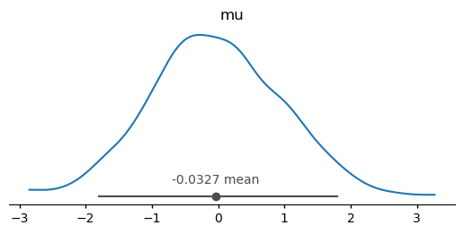
dt = az.load_arviz_data("centered_eight")
az.plot_rank(dt, var_names=["mu", "tau"], backend="matplotlib");

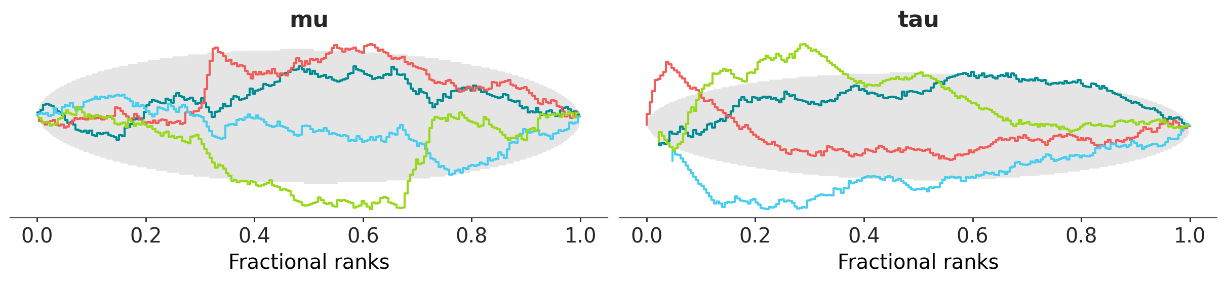
import plotly.io as pio
pio.renderers.default = "notebook"
pc = az.plot_rank(dt, var_names=["mu", "tau"], backend="plotly")
pc.show()

At the time of writing, there are three cross-backend themes defined by ArviZ: arviz-variat, arviz-vibrant and arviz-cetrino.

Plotting function inventory

The following functions have been renamed or restructured:

ArviZ <1	ArviZ >=1
plot_bpv	plot_ppc_pit, plot_ppc_tstat
plot_dist_comparison	plot_prior_posterior
plot_ecdf	plot_dist, plot_ecdf_pit
plot_ess	plot_ess, plot_ess_evolution
plot_forest	plot_forest, plot_ridge
plot_ppc	plot_ppc_dist
plot_posterior, plot_density	plot_dist
plot_trace	plot_trace_dist, plot_trace_rank

Others have had their code rewritten and their arguments updated to some extent, but kept the same name:

• plot_autocorr

• plot_compare

• plot_energy

• plot_loo_pit

• plot_mcse

• plot_rank

The following functions have been added:

• plot_convergence_dist()

• plot_pair_focus()

• plot_ppc_pava()

• plot_ppc_rootogram()

• plot_psense_dist()

• plot_psense_quantities()

• plot_trace()

Some functions have been removed and we don’t plan to add them:

• plot_dist

• plot_kde

And there are also functions we plan to add but aren’t available yet.

• plot_elpd

• plot_khat

• plot_pair

• plot_parallel

• plot_ppc_censored

• plot_ppc_residuals

• plot_violin

• plot_ts

• plot_lm

Note

For now, the documentation for arviz-plots defaults to latest which is built from GitHub with each commit. If you see some of the functions in the last block already on the example gallery you should be able to try them, but only if you install the development version! See Installation

You can see all of them at the arviz-plots gallery.

What to expect from the new plotting functions

There are two main differences with the plotting functions here in legacy ArviZ:

1. The way of forwarding arguments to the plotting backends.

2. The return type is now PlotCollection, one of the key features of arviz-plots. A quick overview in the context of plot_xyz is given here but it later has a section of its own.

Other than that, some arguments have been renamed or gotten different defaults, but nothing major. Note, however, that we have incorporated elements from grammar of graphics into arviz-plots, now that we’ll cover the internals of plot_xyz in passing we’ll use some terms from grammar of graphics. If you have never heard about grammar of graphics we recommend you take a look at Overview before continuing.

kwarg forwarding

Most plot_xyz functions now have a visuals and a stats argument. These arguments are dictionaries whose keys define where their values are forwarded too. The values are also dictionaries representing keyword arguments that will be passed downstream via **kwargs. This allows you to send arbitrary keyword arguments to all the different visual elements or statistical computations that are part of a plot without bloating the call signature with endless xyz_kwargs arguments like in legacy ArviZ.

These same arguments also allow indicating a visual element should not be added to the plot, or providing pre computed statistical summaries for faster re-rendering of plots (at the time of writing pre-computed inputs are only working in plot_forest but should be extended soon).

In addition, the call signature of new plotting functions is plot_xyz(..., **pc_kwargs), with these pc_kwargs being forwarded to the initialization of PlotCollection. This argument allows controlling the layout of the figure as well as any aesthetic mappings that might be used by the plotting function.

For a complete notebook introduction on this see Introduction to batteries-included plots

New return type: PlotCollection

All plot_xyz functions now return a “plotting manager class”. At the time of writing this means either PlotCollection (vast majority of plots) or PlotMatrix (for upcoming plot_pair for example).

These classes are the ones that handle faceting and aesthetic mappings and allow the plot_xyz functions to focus on the visuals and not on the plot layout or encodings.

See Using PlotCollection objects for more details on how to work with existing PlotCollection instances.

Plotting manager classes

As we have just mentioned, plot_xyz use these plotting manager classes and then return them as their output. In addition, we hope users will use these classes directly to help them write custom plotting functions more easily and with more flexibility.

By using these classes, users should be able to focus on writing smaller functions that take care of a “unit of plotting”. You can then use their .map methods to apply these plotting functions as many times as needed given the faceting and aesthetic mappings defined by the user. Different layouts and different mappings will generally not require changes to these plotting functions, only to the arguments that define aesthetic mappings and the faceting strategy.

Take a look at Create your own figure with PlotCollection if that sounds interesting!

Other arviz-plots features

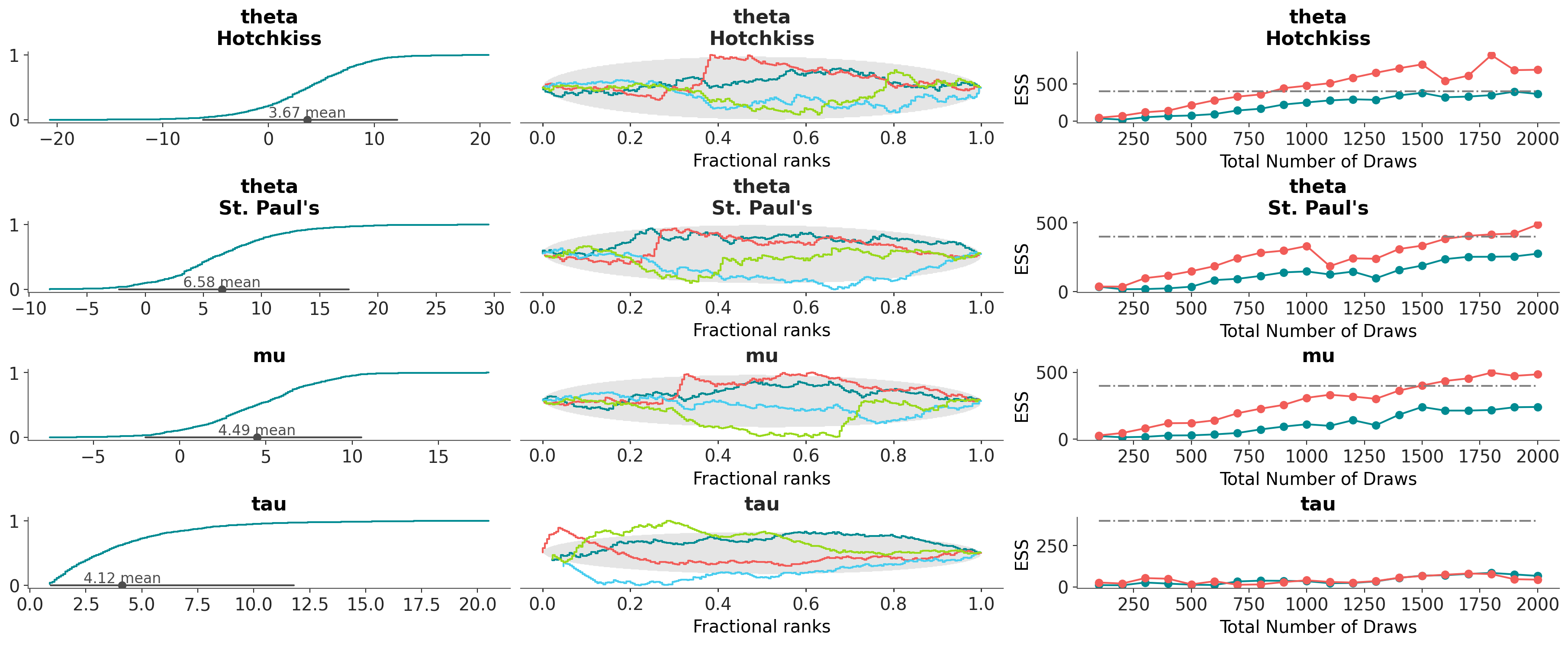
There are also helper functions to help compose or extend existing plotting functions. For example, we can create a new plot, with a similar layout to that of plot_trace_dist or plot_rank_dist but custom diagnostics in each column: distribution, rank and ess evolution:

az.combine_plots(
    dt,
    [
        (az.plot_dist, {"kind": "ecdf"}),
        (az.plot_rank, {}),
        (az.plot_ess_evolution, {}),
    ],
    var_names=["theta", "mu", "tau"],
    coords={"school": ["Hotchkiss", "St. Paul's"]},
)

<arviz_plots.plot_collection.PlotCollection at 0x77b32bc65af0>

---

[1] (1,2)

open_datatree takes an engine argument. Engines “netcdf4” (default if installed) and “h5netcdf” allow reading netCDF4 files. Engine “zarr” should be used to read zarr files.

[2]

User defined modules are valid when doing rcParams["stats.module"] = module but can’t can’t be set as the default through the arvizrc configuration file.